
Multi-armed bandit
This example show how active inference can solve the classic multi-armed bandit problem (MAB). The "bandit problem" refers to classic slot machines invented in the early 20th century which were frequently called "one-armed bandits". The arm refers to the lever on the side of the machine used to spin the reels to initiate a round of play. In this case we will explore a special case known as the two-armed bandit (TAB) problem in which there are two slot machines instead of one (or many).
Bandit problems are popular in many areas of machine learning research because they provide a testbed for models that need to solve problems involving decision-making under uncertainty. Bandit problems are also popular because many real world problems, such as those in operations research, can be reformulated as a bandit problem. Therefore, the bandit problem resembles a very general class of problems with real world relevance.
In this tutorial you will learn:
How to build POMDP models
How to perform action selection in the model editor or the Python SDK
How to interpret the results of action selection
The model file associated with this example is available below:
The problem setup
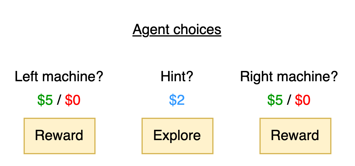
The TAB problem involves two slot machines, each with one arm. We will refer to these machines as the left machine and right machine. During a round of play, the agent has the choice of pulling the handle on either of these machines. When they do so, there is a chance that they may receive a payout of $5 or a chance that they may receive $0. The agent is unaware of the true probability of payout in advance though they may have a good guess. There is also a third option: the agent could ask for a hint. If they do so, they will receive $2 and also learn which slot machine has a higher probability payout. However, taking this hint means that they cannot win a maximum of $5 on this round.
This problem setup presents a scenario in which the agent has two reward-seeking actions it could take - pulling the left machine or the right machine - or a curiosity or exploration based action: getting a hint. The agent's job will be to balance these actions in order to maximize its overall profit. In some situations it may be better to activate a slot machine and try to get a reward. In other cases, the agent may want to get a hint to better understand its environment first so that it can more confidently activate the correct machine and maximize its probability of payout.
As mentioned in the tutorial on active inference, we will see that active inference agents can solve the TAB (or MAB) problem without being explicitly programmed to explore or seek rewards. We merely need to set up a model and present the agent with an observation and it will determine the best sequence of actions needed to attain its goals. We are now in a position to define the problem statement:
Problem statement: Given two slot machines with a possible payout of $5 and the ability to get a hint about which machine is better (with a 100% chance of receiving $2) what is the best sequence of actions to take to maximize profit?
The active inference agent
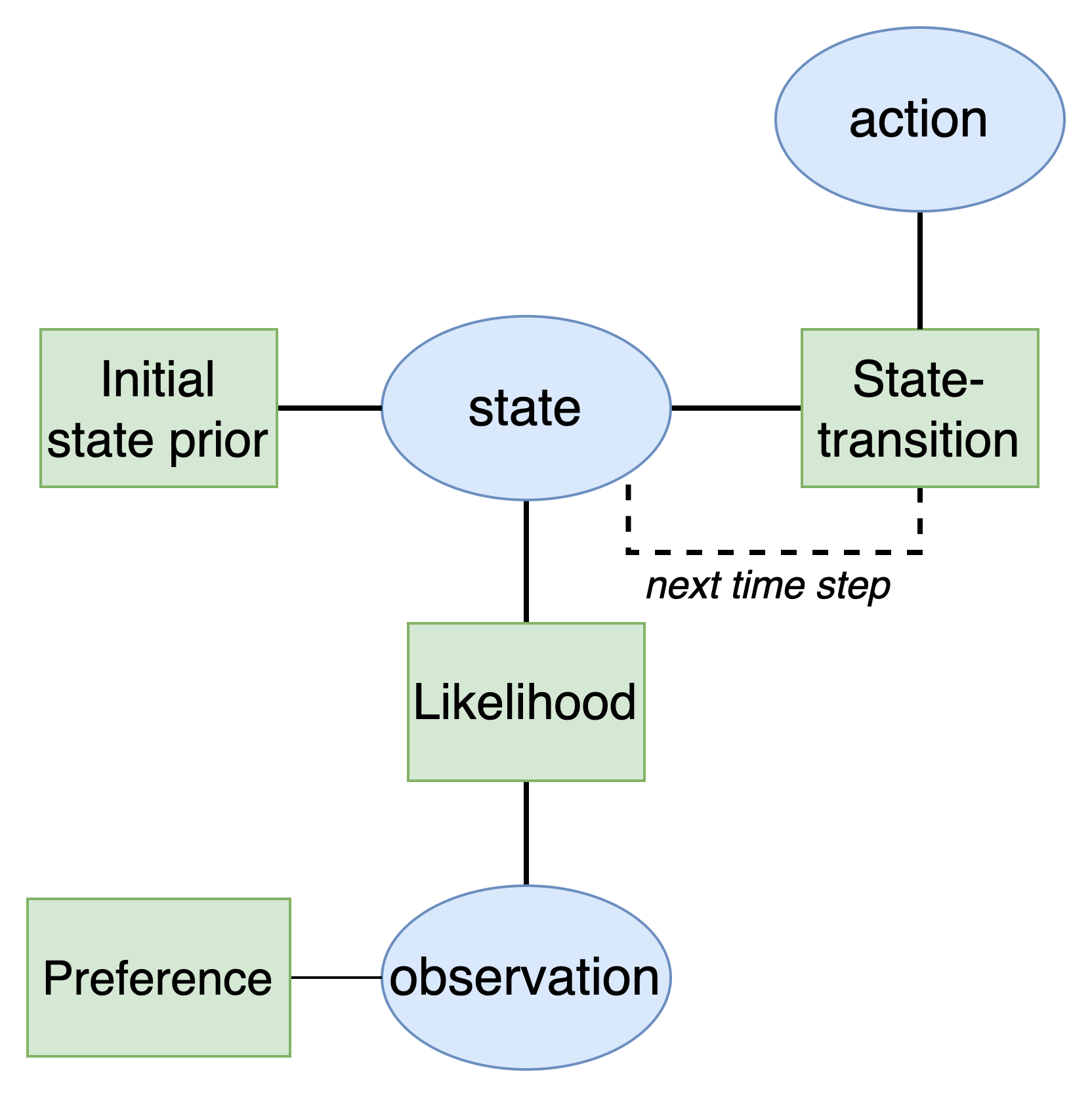
The first goal will be to develop an active inference agent. As explained in the active inference tutorial, active inference agents utilize a Bayesian network with a special structure known as a partially observable Markov decision process (POMDP). This model has the following structure:
Defining the states and observations
Our next goal is to define the model variables we will use in the model. First, we need to define the model states and observations (also known as data or evidence). Unlike the agent navigation example, the POMDP model for the TAB problem will be much more complex. We will have multiple different types of states known as state factors and multiple types of observations/data known as observation modalities. This simply means that there are multiple groups of states and observations instead of a single one in the agent's model.
State factor 1: Context
The first state factor is named context. This state captures which machine gives a payout of $5 over the course of the experiment.
Left-better
The left machine will win
Right-better
The right machine will win
State factor 2: Choice
The second state factor is named choice. This state captures the actions the agent can make.
Start
The simulation is in the starting state
Hint
A hint was taken
Left-arm
The left machine was activated
Right-arm
The right machine was activated
Observation modality 1: Hint
The first observation modalities is named hint and captures the observations that result from taking a hint.
Null
No hint was taken
Hint-left
Hint says left machine is better
Hint-right
Hint says right machine is better
Observation modality 2: Reward
The second observation modality is named reward and captures the observations that result from receiving a reward or not.
Null
No reward was received (start of simulation)
Loss
A loss was received
Reward
A reward was received
Observation modality 3: Choice
The third observation modality is named choice and captures the observations that result from making a choice.
Start
Agent is starting simulation
Hint
Agent took a hint
Left-arm
Agent activated the left arm
Right-arm
Agent activated the right arm
Defining actions
Additionally, the agent can take multiple possible actions. Since actions are directly connected to controlling states, the agent needs two ways to represent its possible actions in connection to each state factor (Choice and Context).
Action set 1: Context
This action set represents how the agent can alter the context - which machine is better. We will assume that the agent is not able to control this aspect of its environment which is true of real slot machines.
Do-nothing
The agent does nothing to change context
Actions set 2: Choice
This action set represents the choices the agent can make at each time step to affect environment states.
Move-start
Start the simulation
Get-hint
Get a hint
Play-left
Activate the left machine
Play-right
Activate the right machine
Defining the model factors
Next we define the model factors. The likelihood defines how the agent's beliefs about states generate observations. Unlike the agent navigation example, we now have multiple states to account for with each possible observation. In other words, since there are three possible observations sets (hint, reward, choice) each will have an independent likelihood associated with it that shows what combination of states could generate this observation.
Likelihood 1: Hint observation modality
This likelihood represents the likelihood of receiving a hint given the context the agent is in (Left-better, Right-better) and the possible choices (Start, Hint, Left-arm, Right-arm). We must define a probability for each of these combinations. They will be as follows:
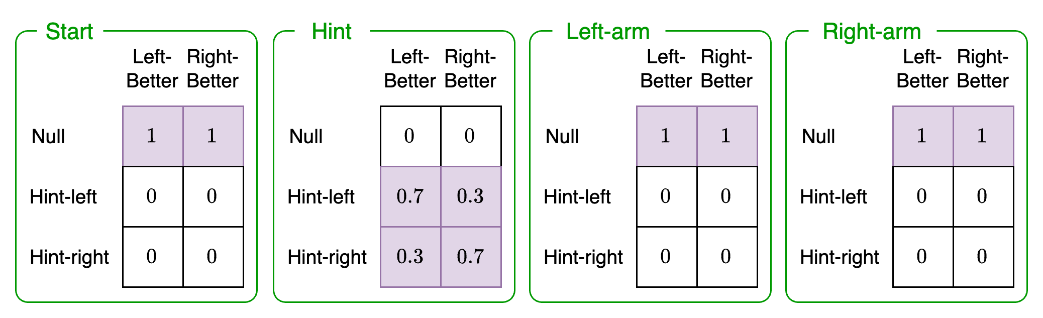
The green box indicates state factor 2: choice. The columns show state factor 1: context. The rows of each matrix indicate the hint observation modality. In other words, this likelihood enumerates all the different probabilities for what the agent believes for the choice state factor, context state factor, and resulting hint observation.
To understand what these matrices represent, let's take an example. The second green box, row 2, column 2 denotes the following categories:
Hint observation: Hint-left (row 2)
Context state factor: Left-better (column 2)
Choice state factor: Hint (second green box)
Navigating to this entry in this matrix we see that it is 0.7. This means that if it were the case that the left machine was better and a hint was taken, then the agent would expect to learn that the left machine is better with a probability of 0.7.
Likelihood 2: Reward observation modality
This likelihood represents the likelihood of receiving a reward given the context the agent is in (Left-better, Right-better) and the possible choices (Start, Hint, Left-arm, Right-arm):
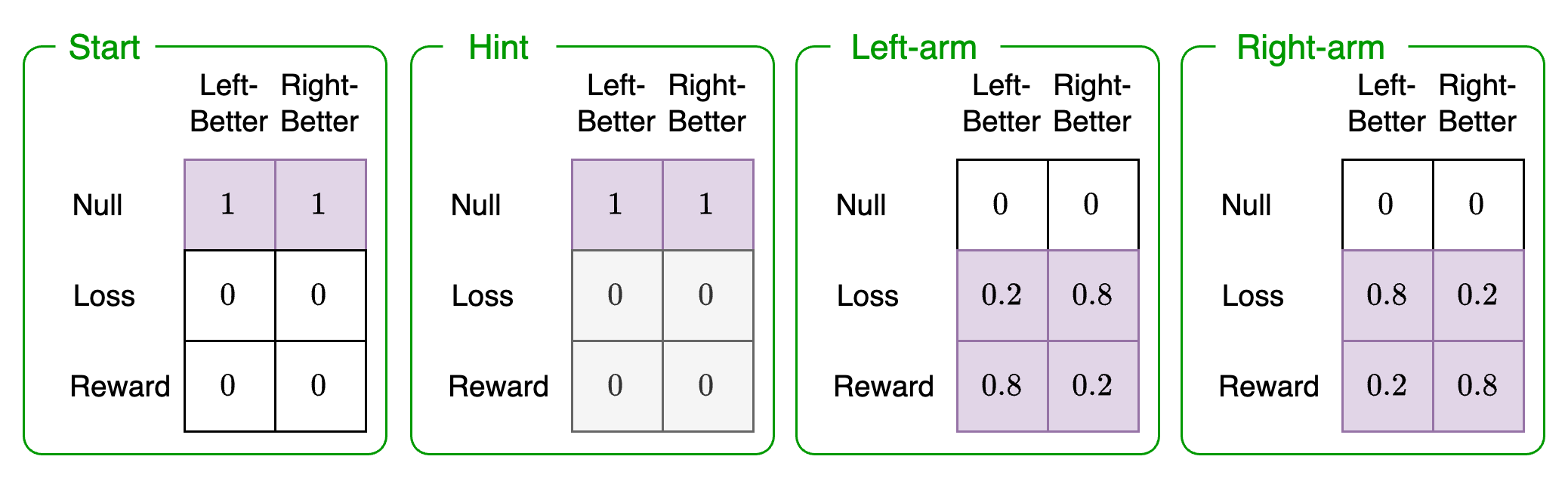
For example the thrid green box, row 3, column 1 denotes the following categories:
Reward observation: Reward (row 3)
Context state factor: Left-better (column 1)
Choice state factor: Left-arm (third green box)
The entry in the matrix for this combination is 0.8. This indicates that if the agent believed that the left machine was better and it activated the left arm, it would expect to receive a reward with a probability of 0.8.
Likelihood 3: Choice observation modality
This likelihood represents the likelihood of seeing a particular choice given the context the agent is in (Left-better, Right-better) and the possible choices (Start, Hint, Left-arm, Right-arm):

This likelihood just captures the agent's awareness of its own choices. If it took a hint then regardless of which machine it believes is better, it would expect to receive an observation that it took a hint. The same applies for the other categories. This just implies that the agent has some way of knowing or observing its own actions (for example, visual cues).
Transition 1: Context state-transition
The context state-transition captures the probability of transitioning to a different state given that the agent performs the Do-nothing context action.
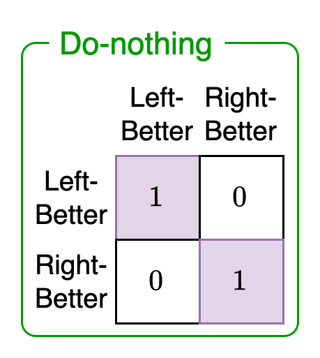
This action just encodes the fact that the agent cannot change the context of the game. In other words, it cannot control the slot machine probabilities and force one to be more likely to payout than the other. Since all state-transitions must be associated with an action, the Do-nothing action will result in an identity matrix where the state at the current time step (columns) will stay the same at the next time step (rows).
Transition 2: Choice state-transition
The choice state-transition captures the probability of transitioning to a different state given that the agent performs the the Move-start, Get-hint, Play-left, or Play-right actions:
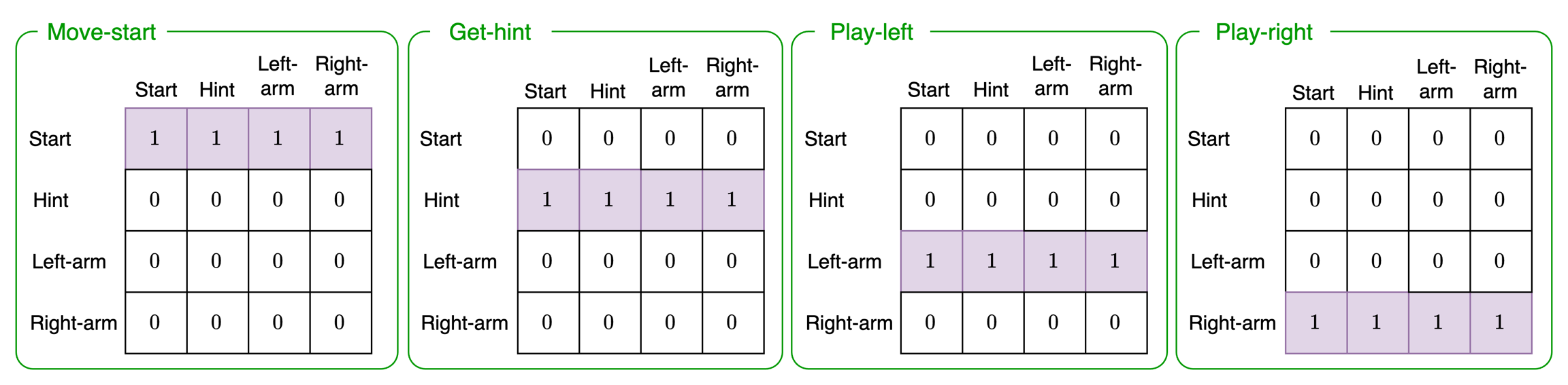
All these matrices encode is the fact that when an agent performs a particular action, it expects the action to take place regardless of what the past state was. For example, if the agent chooses to Play-left (third green box), then regardless of what the past state was (columns) the agent expects to activate the left-arm (row three, all probability of 1).
Initial state priors: Choice and context
We have two different types of state factors - choice and context. Therefore, we need separate initial state priors for both of these.
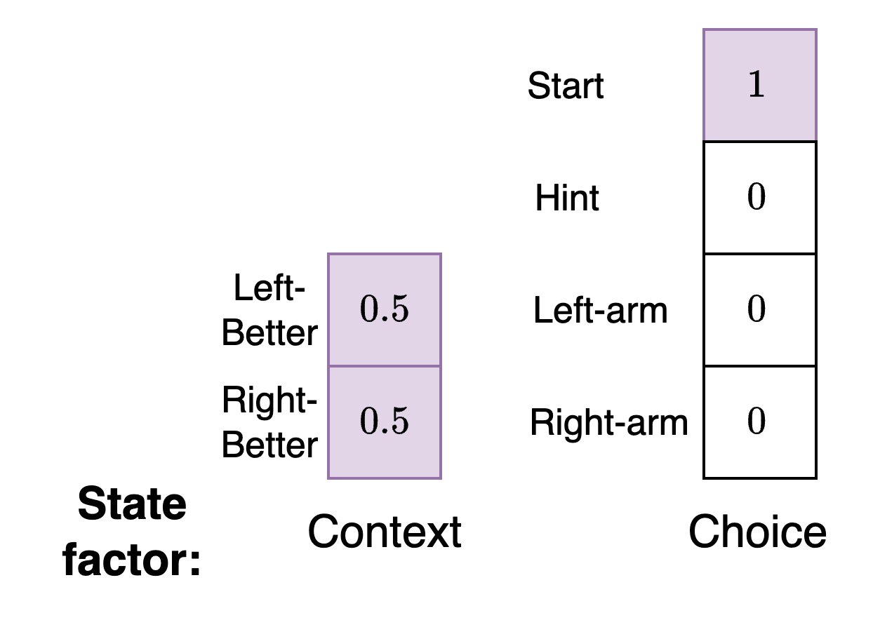
For the context state factor we see that at the start of the simulation the agent does not consider either the left or right arm to be better. For the choice state factor the agent expects to begin in the starting state of the simulation.
Preferences: Hint, reward, and choice
We have three different types of observation modalities - hint, reward, and choice. Therefore, we need separate preferences for each.
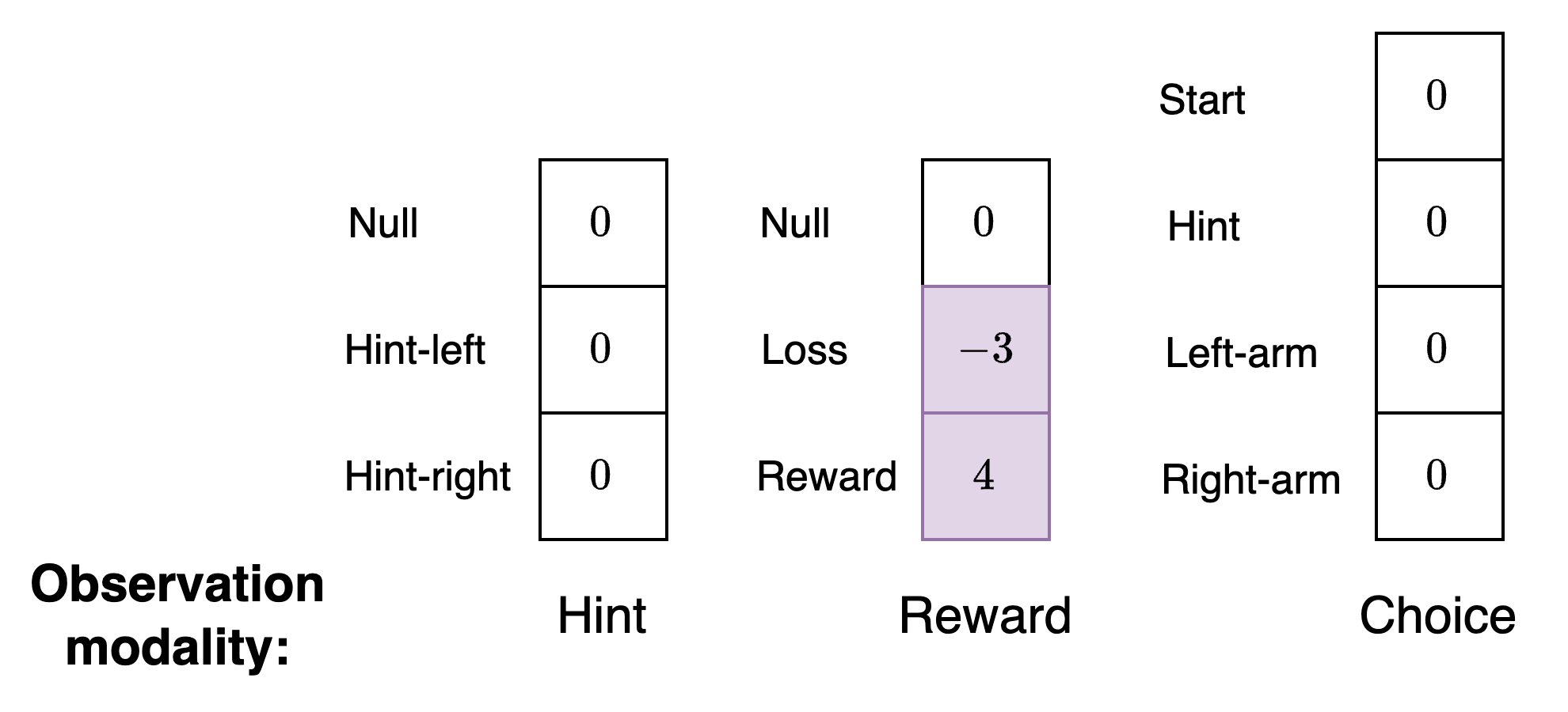
For the hint and choice observation modalities, the agent will not have any preferences. Instead, the agent just needs preferences for the type of reward it wishes to receive from the environment. You will notice that this vector is not a valid probability distribution. This vector will be converted into a valid probability distribution by the Genius agent.
Since it is more natural for us, as designers of models, to think in terms of positive and negative values for preferences and aversions instead of probabilities we allow preferences to be specified in this way.
Visualizing the full model
For the TAB model we have presented here, the POMDP has a much more complex structure than the simpler one found in the agent navigation example:
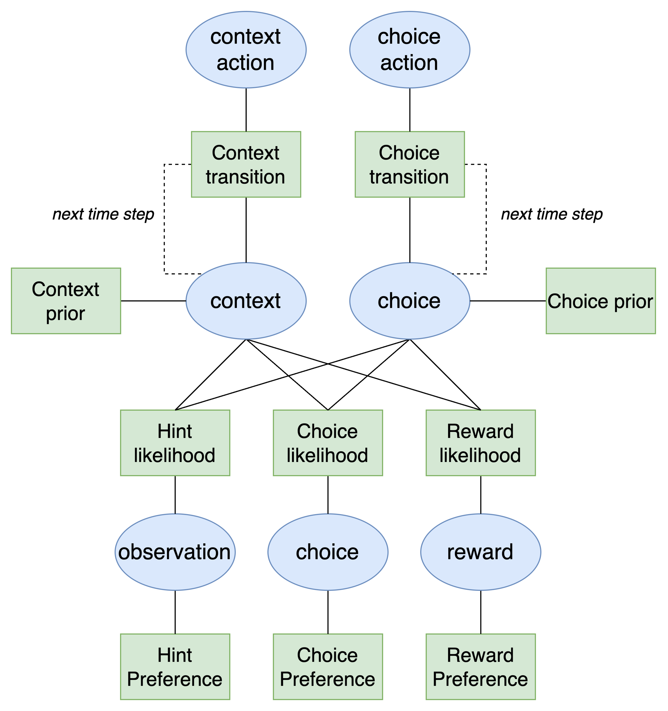
As we can see, the presence of multiple state factors and observation modalities means that we need extra branches in the model to account for them. Ultimately, the model is essentially the same as the simpler model but we have two new branches for each state factor (both of which transition over time) and three new branches for each of the observation modalities and their associated preferences.
The action-perception loop
The action-perception loop specifies how the agent interacts with its environment. Each time the agent executes an action it will alter the environment by activating either the left or right arm of the bandit machine. This will change the state of the machine which in turn will lead to a new observation generate. A full step of the simulation would consist of the following steps:
Agent:
Receive hint, reward, and choice observations from the bandit machine
Use observation to determine a belief about the current context and choice state factors of the environment (perception)
Determine the correct action to take based on prior preferences (decision-making / action selection)
Execute action
Environment (bandit machine)
Receive action from agent
Use action to transition true context and choice state factors of the environment
Generate hint, reward, and choice observations based on the next state of the environment
Repeat steps 1 and 2
Querying the model
In this section we demonstrate how to perform active inference in the model editor and the Python SDK.
To query the model, we need to first connect to the agent, load a JSON model file, and send the loaded model to the agent. We will use the multi-armed bandit POMDP file which can either be pasted into the box during loading or saved locally. After these steps are done, we are ready to query the agent.
To perform active inference in this scenario we will need to act as the bandit machine and simulate one step of the environment. For example suppose the agent observes the following:
Hint = Null
Reward = Loss
Choice = Left-Arm
This means that it did not take a hint. But in the previous round it received a loss ($0) and picked the left-arm. Let's examine the agent's selected action for this step of the action-perception loop. To do so, we go to the Action Selection panel and select the radio buttons corresponding to the observations in the bullet list above. Then we click "Run". The results:
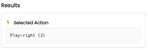
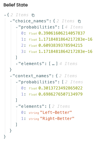
As we can see, the agent has chosen Play-Right as its action. According to the agent's output, we can see that it currently believes that the right slot machine is better.
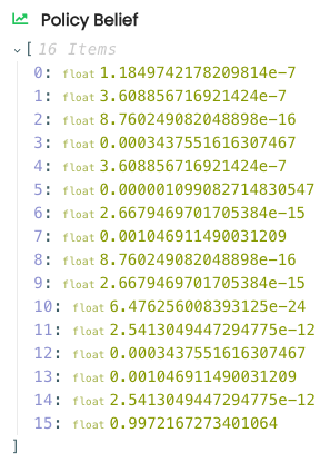
Finally, examining the policy probabilities we see that the last policy, corresponding to the action sequence Play-right, Play-right had the highest probability of being chosen:
First, we import the necessary modules:
After connecting to the agent, we can build the Genius agent. If we have a POMDP model available we can just import it to the GeniusAgent class. However, here we show how to build the model from scratch. First, we initialize the POMDP model:
Now we set the names for the states, observations, and actions. We then add them to the model we are constructing.
Next, we create the factors. We need to specify both the names of the variables that the factor is connected to and the corresponding probabilities. We can then add them to the POMDP model we are constructing.
Now we create a Genius agent and load the model into the agent.
Next, we need to define the environment. This environment will act as the actual slot machine which responds to the agent's possible actions and generates a result.
Next we initialize the simulation setup. Here we assume that the accuracy of the hint is perfect. We could modify this if we would like to see how the agent performs under conditions where a hint is not completely accurate. We assume that the true probability of reward is 0.7. Note that this is slightly different than the agent's believe about the probability of reward which is 0.8 as specified in the reward observation modality.
We will run the simulation for 15 time steps and specify that the agent plans ahead two actions into the future at each time step. Finally, note that according to this environment, in reality the left slot machine is better.
Context: Left-Better
We also define two helper functions. The first function will help us parse through the result of action selection to pull out the state the agent believes is mostly likely having seen the data at each time step. The second function updates the model with this new state belief.
Next we initialize the first observation ourselves. At the beginning of the experiment the only thing the agent observes is that it has started the experiment. Hints and rewards must be null if the agent has not begun the simulation.
Lastly, we need to store the history of actions. We also store the prior context values for the 0th time step so we can plot them later.
Now the simulation loop can be specified. We perform the following steps:
The agent performs an action given an observation for each modality. We then print out the most likely state belief that is inferred for each state factor using the observation modalities.
The agent's chosen action index is recorded and converted into its string representation.
The state factor belief probabilities are extracted and used to update the model.
The environment is given the agent's chosen action index which causes each state factor to transition to the next state. As a result of this transition, a new observation is generated.
The chosen action and reward are recorded and history is updated.
A partial view of the printed output during the simulation is show below:
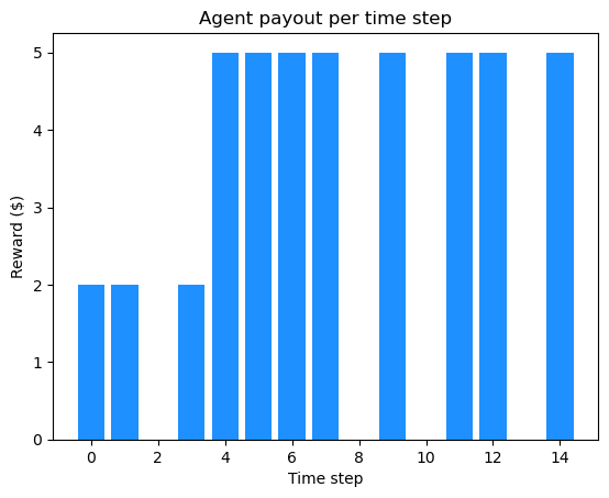
At the end of the experiment, the agent maximizes its reward with a cumulative payout of $45. When we break this down into losses and gains per time step we see the following:
Interpreting the results
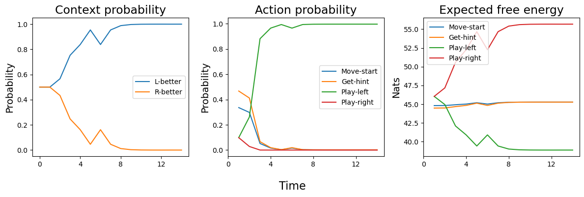
Below we gather the context state belief, action probabilities, and expected free energy for each time step and plot them.
Left panel: The agent starts out with a uniform belief that either the left or right machine could be better. After roughly 10 time steps, the agent believes that the left machine is better with a probability near 1. This matches the true state of the environment - the left machine was better in this simulation.
Middle panel: The agent starts out with a high probability of getting a hint. The hint is immedietly informative to the agent and enables it to quickly determine that the left machine is better. Thus, all other actions become unlikely to be selected and drop toward zero and the
Play-leftaction becomes dominant.Right-panel: The agent's expected free energy corresponds closely to the action probabilities over time. Recall that agents will select policies with the lowest EFE. We can see here that the EFE for the
Play-leftaction drops over time which means its is more likely to be selected at each time step over the other actions. Early on, there is a higher chance of getting a hint but as soon as this hint is informative, it is not longer as probable asPlay-left. This can be seen in the plot around time step 3 when thePlay-leftEFE drops below theGet-hintEFE.
As we can see, the agent quickly determines which machine gives a better payout. We can easily manipulate this agent and see how it responds to other scenarios. For example, we could make it risk-averse so it is less likely to take hints. We could also alter the probability of hint accuracy so that the agent operates under further conditions of uncertainty. Both of these scenarios would result in an agent that would take longer to determine which machine is better and maximize its payout.
Last updated