Discrete Bayesian networks

To demonstrate how Genius agents reason under uncertainty we will introduce a simple example of a Bayesian network. Bayesian networks are described by a type of graph known as a directed acyclic graph (DAG). Consider the Bayesian network below which is an example from the sprinkler dataset.

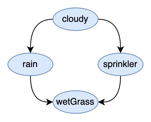
Bayesian network for the sprinkler dataset

The type of probabilistic graphical model shown here is a Bayesian network which captures the dependencies between discrete variables of interest in our model. The circles that contain the variables are known as nodes or vertices in the graph. Each variable is discrete because it stores different, individuated categories of interest.

Variable	Categories	Description
cloudy	yes, no	Is it cloudy?
rain	yes, no	Is it raining?
sprinkler	on, off	Sprinkler state
wetGrass	yes, no	Is the grass wet?

In other words, each variable can be broken down into categories which, in this example, indicate a status or "state".

The lines in this graph are called edges. Specifically, these are directed edges because the lines have arrowheads on them. These directed edges specify the dependency among the variables of the model. This introduces structure into the model that captures the relationship between variables of some real world process. The world itself is structured, usually through cause and effect, and the dependencies may capture these relationships. The major constraint on the structure of Bayesian networks is that there are no loops in the directed edges that connect the nodes (e.g. the graph is acyclic).

The sprinkler model shown above tells us the grass being wet or not (Yes/No) depends on the state of the sprinkler (on/off) and whether it is raining (yes/no). In turn, being rainy or not depends on if it is cloudy (yes/no) and whether or not a sprinkler is on or off depends on if it is cloudy (Yes/No).

As we can see from this simple example, this graph captures the logical chain needed to reason about whether or not the grass is wet. But how does uncertainty come into play?

Capturing uncertainty with probability

To capture uncertainty, we need to introduce the notion of probability and apply it to the variables of interest in the model. Now the relationships among the variables will be represented by a value, between 0 and 1, representing the probability of the different possible interactions among the categories of the model, as explained below.

Representing uncertainty in terms of probability naturally means we are working with a levels of confidence in a particular state of the world being the case. It is customary to refer to these levels of confidence with the metaphor of degrees of belief about a state. For many models of the real world we cannot be certain of all the possible states and assign a probability to it. For example, in the case of medical diagnosis, we could not enumerate all possible symptoms for all possible diseases.

However, we can often simplify by only considering a subset of variables that are likely to be relevant while others may be considered low probability. Deciding how to represent the process being modeled probabilistically is key to the design of a good model. A good model should not literally recapitulate every detail of the world deterministically but provide the "least you need to know for accurate predictions" approximation.

In many cases, we can get away with a lot of simplification. As we will see below, this is certainly the case with the sprinkler example. Although we could choose to divide the status of "cloudy" and "rain" into further categories rather than just a simple binary, adding this extra detail is unlikely to make the prediction of wet grass more accurate. The simple model is also much easier to understand and interpret. We will assign the following probabilities to each variable in the model:

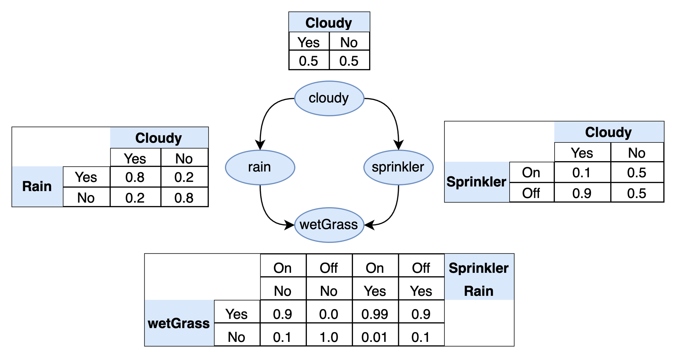
Bayesian network for sprinkler dataset with associated probabilities

As we can see, we have enumerated all possible combinations of states for each variable under consideration and the expected probability of the outcome. Using this table, it is now possible to ask questions like:

• What is the probability that it is cloudy? Looking at the top table, this is 0.5, which also happens to be the same probability that it is not cloudy. This is an example of a marginal probability (also known as a prior probability) whose values do not depend on the state of any other variable in the model (i.e. they are independent of these other variables).

• What is the probability that it is not cloudy but it is rainy? Looking at the left table this 0.2.

• What is the probability that it is cloudy but the sprinkler is off? Looking at the right table this is 0.9.

Asking more complex questions will become tedious to do by hand which is why will introduce the notion of probabilistic inference which will allow us to query the probability over any variable in our Bayesian network given what data we observe.

Notice variables with dependencies get extra column headings in the table. This allows us to take into account the fact that the probability of a variable may change depending on the state of the variable it depends on. For example, the probability of it raining will change depending on whether or not it is cloudy. The extra column in the table takes account this fact. This is known as a conditional probability.

"wetGrass" depends on two variables and we therefore need to enumerate all possibilities of both variables it depends on: "sprinkler" and "rain". In general, the number of probabilities we need is equal to the Cartesian product of the number of categories for the variables involved. Since there are two binary variables with two categories each, there will $2 \times 2=4$ possibilities to consider which corresponds to the four rows in the bottom table. Enumerating the probabilities for all combinations of states in this way also reveals the notion of independence. For example, "sprinkler" does not depend on "rain" and is therefore independent of rain in this model.

In short, this simple model allows us to reason, under conditions of uncertainty, about whether or not the grass will be wet given other factors we are considering that we belief results in wet grass.

The distributions in this table must satisfy two important axioms of probability:

• Each column is a categorical distribution, specifically a binary categorical distribution in the sprinkler example, and so these columns must always sum to one.

• Probabilities must always be between 0 and 1, inclusive.

Probabilistic notation

When one queries a probabilistic model they will typically use specific mathematical notation. The queries in the previous section omitted this notation. To notate probability we use the symbol capital $P$ which indicates a probability mass function. This is followed by parentheses and then the variable(s) of interest. For example, the probability of it being cloudy is $P(cloudy)$. If we wish to denote a dependency we can use the $\mid$ symbol. The probability of rain given that it is cloudy is $P(rain \mid cloudy)$. If a variable depends on multiple variables, they are separated by a comma. Taken together, the four distributions in our model are

$$\begin{aligned} P&(cloudy) \\ P&(rain \mid cloudy) \\ P&(sprinkler \mid cloudy) \\ P&(wetGrass \mid sprinkler, rain) \end{aligned}$$

The product of these four distributions is the joint probability distribution of the variables of interest, also known as a probabilistic model:

$$P(cloudy, rain, sprinkler, wetGrass) = P(cloudy) \times P(rain \mid cloudy) \times P(sprinkler \mid cloudy) \times P(wetGrass \mid sprinkler, rain)$$

Finally, if we wish to query the model, we can specify the value or evidence for the variable in question. This evidence corresponds to the data we have available to us that we collect from the real world. For example, $P(rain \mid cloudy = yes)$ can be read as "what is the probability of rain given the evidence that we observe it is cloudy?" The answer, according to the table, is a 0.8 probability that it is raining and 0.2 probability that it is not. For a more complex example, $P(wetGrass \mid sprinkler = on, rain = no)$ may be read as "what is the probability that the grass is wet given the evidence that the sprinkler is on and there is no rain?" According to the table, there is a 0.9 probability that the grass is wet and 0.1 probability that it is not.