
Agent navigation
In this tutorial we show how to perform active inference in a simple agent navigation model. In the explanation of active inference given in a previous tutorial we emphasized the fact that active inference agents need an environment to interact with. We will use the classic GridWorld environment to demonstrate agent navigation.
In this tutorial you will learn:
How to build POMDP models
How to perform action selection in the model editor or the Python SDK
How to interpret the results of action selection
The model file associated with this example is show below:
The GridWorld environment
In GridWorld, an agent inhabits a simple environment consisting of 9 squares:
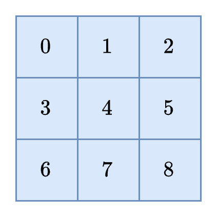
The agent will start the simulation in one of these nine squares. The agent's goal is then to navigate to another square on the grid. To make this example more realistic, let's suppose that these squares correspond to physical locations or areas of a large, simplified model of a real world warehouse. Below is a list of each of these locations and the corresponding description:
0
Loading dock (load)
A large area near the entrance where goods are loaded and unloaded
1
Aisle near shelving units (aisle)
An aisle between rows of storage shelves
2
Bulk storage (store)
A large open space or room where large or bulk items are stored on pallets
3
Inventory office (office)
An office or small room where warehouse operations are monitored and controlled
4
Conveyor belt area (convey)
A section of the warehouse with moving conveyor belts used to transport items
5
Forklift charging station (charge)
A designated area where forklifts are recharged or stored when not in use
6
Packing station (pack)
An area where goods are being packaged or processed, with tables and packing materials
7
Shipping and receiving desk (desk)
An office or small room where warehouse operations are monitored and controlled
8
End of aisle (end)
A location near the end of a particular aisle that may have exits or walkways leading outside
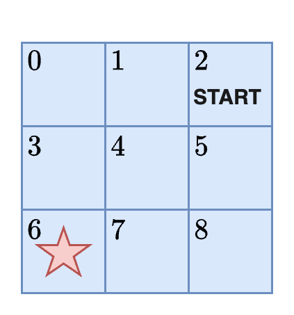
Problem statement: If the agent begins in bulk storage (position 2) how can it get to the packing station?
According to this problem statement, the agent must begin at the START and navigate to the red star:
The active inference agent
The first goal will be to develop an active inference agent. As explained in the active inference tutorial, active inference agents utilize a Bayesian network with a special structure known as a partially observable Markov decision process (POMDP). This model has the following structure:
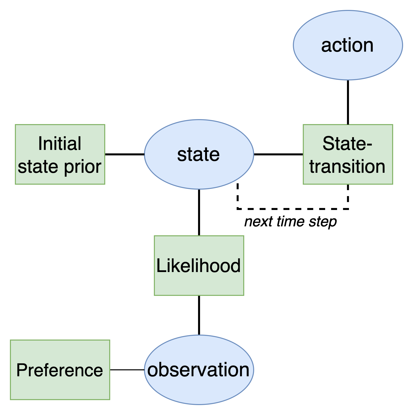
Defining the model variables
Creating an active inference agent therefore involves defining the structure of the variables and factors in the model. Since we are operating under assumptions of partial observability, the agent would not know its actual position in the warehouse at any given moment in time. All it has access to are its sensors which stream in data that we will call the agent's observations. The agent must use these observations alone to infer its actual position in the environment. We can think of the observations as context clues that uniquely identify its position. With this in mind, we can define our states and observations.
States: The agent's position in the warehouse which will change over time as it moves. The position variable will have nine categories in it corresponding to the unique warehouse locations.
State: The agent's belief about its position in the warehouse which will change over time as it moves.
Observations: What the agent observes when it is in a particular position in the warehouse. These observations can help the agent identify where it is because certain features of its world (the warehouse) are associated with its position. For example, when the agent is in the state
aisleit would expect to observeshelves.
load
door
A large overhead door with a textured ramp
aisle
shelf
Rows of shelves filled with boxes or goods
store
pallet
Large stacks of pallets on industrial shelves
office
table
Tables and desks with packing tape and materials
convey
belt
Boxes moving on a belt
charge
light
Forklift charging lights
pack
box
Boxes being packed
desk
paper
Desks with paperwork and packing lists
end
ramp
A large concerete ramp
It is important to note from these observations that the agent may not be able to uniquely identify its position from the observation alone. For example, multiple positions are associated with shelves, desk, or ramps. This is not a problem in itself as it reflects a situation of decision-making under uncertainty.
We also need to select the possible actions the agent can perform in this environment. We will assume that the agent has five possible options. It can move UP, DOWN, LEFT, RIGHT, or STAY in order to move between the different warehouse locations.
Defining the model factors
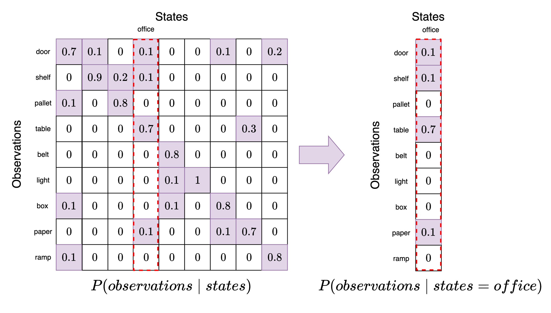
Now our goal is to set the model factors. The model factors capture the probabilities in the model that relate the model variables. We start with the likelihood which defines agent's belief about how states generate observations. In other words, if the agent is in a particular state (position in the warehouse) what does the agent believe is the probability of receiving a particular observation (sensor data)? This can be compactly represented in a likelihood tensor which represents a piece of the agent's understanding about the structure of the world. We will use the following likelihood tensor:
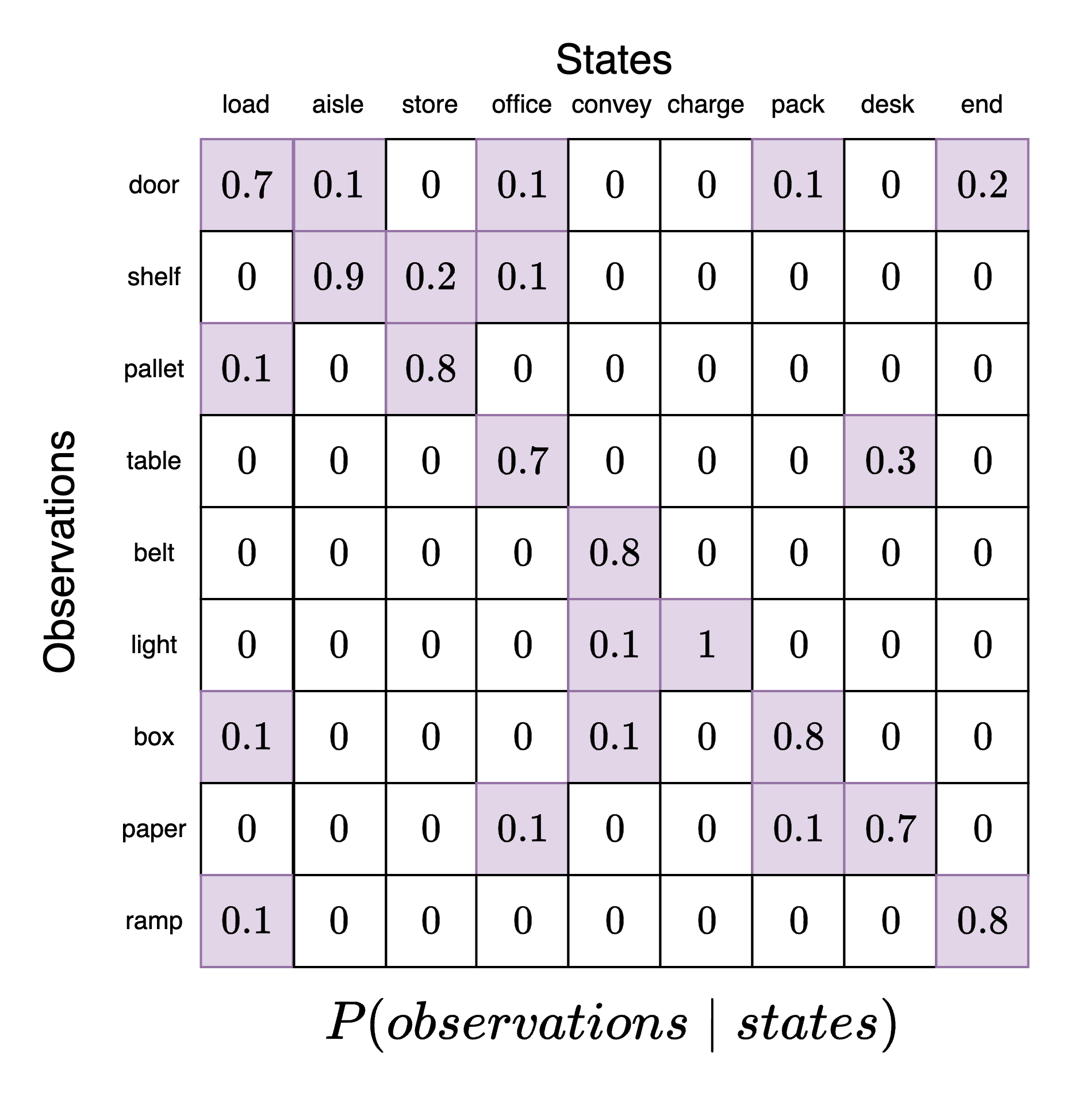
This likelihood tensor has the state categories along the columns and the observation categories along the rows. Each column is a categorical distribution that must sum to 1. As we can see, the agent has the highest probability of identifying the correct association between a state and the resulting observations (main diagonal of the likelihood tensor, top-left corner to bottom-right corner). However, there is a small probability that the same state is associated with other observations.
For example, suppose the agent believes it is in position 3 (office). To see what observations it believes are most likely, we take this slice out and examine it. Each element in this slice now corresponds to a particular observation category where have locked in state=office. We can see here that the observation category table has a probability of 0.7. This means that when an agent is in the office it expects to see a table with the highest probability. However, it may also expect to see paper, shelves, or a door.
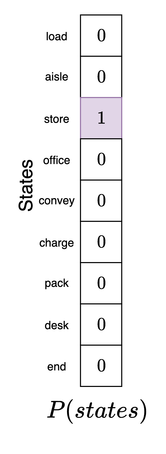
Next, we define the initial state prior factor. This is the agent's belief about its position at the beginning of the experiment. We are free to specify this model component as we like for the simulation. We will assume that the agent (correctly) believes that it is in its actual starting position in the packing area. We indicate this by creating a state vector where each element corresponds to the agent's belief about what position it is in and mark the packing area with a 1. This denotes completely certainty by the agent about where it is. Note that this may not be where the agent actually is, just where it believes that it is before it has seen any data to confirm or deny this initial hypothesis.
Next, we need a state-transition factor. This factor specifies how the agent believes the environment will change over time given a particular action it performs.
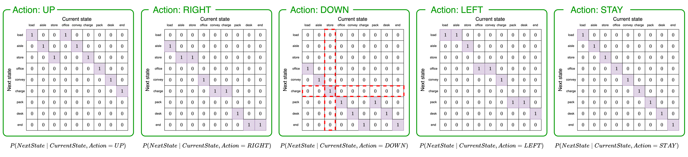
The above five tensors represent "slices" of the full state-transition tensor, one for each possible action. To determine the agent's belief about the next state of the environment, the agent will follow these steps:
Determine the action the agent will perform. We will say the agent is going to move DOWN. If the agent is moving DOWN it will use the third tensor to determine the next state (green box with
Action: DOWN).Determine the agent's current belief about its position. We will say the agent believes it is in position 2 (
store). We use this to pick the second column of the matrix (vertical red box).Determine the probabilities of transitioning to the next state. According to the column we selected in step 2, the agent believes it has a probability of 1 of transitioning to position 5 (
charge).
In the agent's model, the five slices of the state-transition tensor would be combined into a single object rather than five separate objects as shown in the figure.
Finally, we need a preference factor. This preference factor encodes the agent's "desire", "goal", or, more accurately, expectations about the types of observations it wishes to receive from the environment. Not that we define preferences here in terms of the observations the agent expects to receive and not the state it desires to be in. For this example, the agent desires to be in the packing station, pack. So, it would expect to receive observations that indicate it is in this position (box):
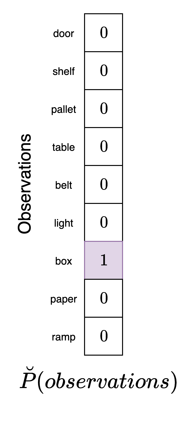
This vector has a "1" in the entry corresponding to box which indicates that its goal is to receive observations from the environment correspond to boxes. Note that according to the agent's model, boxes are most highly associated with the packing area which is the position it would end up in if it pursued actions that would bring about the highest probability of observing boxes. However, there are other positions it could be in within the warehouse that would also result in this observation. This fact once again highlights that the agent must make decisions under conditions of uncertainty.
The action-perception loop
As indicated in the previous active inference tutorial, the agent uses its model to select sequences of actions to obtain its goal. Each time it executes an action it will alter the environment (its true position) which will lead to a new observation being generated. A full step of the simulation would consist of the following steps:
Agent:
Receive observation from warehouse environment
Use observation to determine a belief about the current state of the environment (perception)
Determine the correct action to take based on prior preferences (decision-making / action selection)
Execute action and move to new position in the warehouse
Environment:
Receive action from agent
Use action to transition to a new state (state-transition)
Generate observation based on this new state
Repeat steps 1 and 2
This is sometimes referred to as the action-perception cycle in the active inference literature. In our particular example, this process entails the following:
The agent determines its position in the warehouse from observation received in the environment
The agent uses its preferences to decide and execute an action that will bring it closer to its goals
The environment (the agent's position) changes to a new state as a result of the action
This new state generates new observation that the agent can receive
Querying the model
In this section we demonstrate how to perform active inference in the model editor and in the Python SDK.
To query the model, we need to first connect to the agent, load a JSON model file, and send the loaded model to the agent. We will use the GridWorld POMDP file which can either be pasted into the box during loading or saved locally. After this is done, we are ready to query the model.
To perform active inference in this scenario we will need to manually specify the agent's new position given the action they perform. At the start of the simulation, the agent believes that it is in position 2 (store) which means that they are the storage area. Since the agent really is here (its beliefs conform with reality) it will receives the pallet observation when in this part of the warehouse. We provide this observation to the agent and examine the result:
If the agent moves left, it will be in the aisle position. The correspond observation it would receive here is shelf. We provide this observation to the agent and see that the selected action is DOWN which moves it into the convey position.
From here, the agent receives the belt observation and selects the DOWN action. This brings it to the desk position where the agent receives the paper observation. Continuing in this fashion we see that the agent makes its way to the final pack position where it performs the STAY action.
First, we import the necessary modules:
After connecting to the agent, we can build the Genius agent. If we have a POMDP model available we can just import it to the GeniusAgent class. However, here we show how to build the model from scratch. First, we initialize the POMDP model:
Now we set the names for the states, observations, and actions. We then add them to the model we are constructing.
Next, we create the factors. We need to specify both the names of the variables that the factor is connected to and the corresponding probabilities. We can then add them to the POMDP model we are constructing.
Now we create a Genius agent and load the model into the agent.
Next, we need some helper functions. The first will be a function that defines the environment. This function will, at each time step, use the current position to transition to a new position and then generate observations from this position. This can be achieved with matrix multiplication between vectors that encode the position, a likelihood matrix, a transition matrix, and a chosen action:
We also create a helper function that will allow us to update the model after the state has been inferred.
Next, we set up the simulation. To do so, we first need to specify the starting position (position 2). We also specify the number of time steps in the simulation and possible action names. We also specify the policy length - that is, the number of steps ahead into the future the agent will plan. We have chosen a small policy length of 2.
Active inference agents will perform an exhaustive search of all possible combinations of policies possible. This can quickly become computationally expensive so it is advisable to limit the policy length to less than 5 for most models.
Now we can run the active inference model for the n_steps time steps. At each time step, the environment transitions to a new state and generates an observation. We print out the new environment position and then use the Genius active inference agent to generate an action. This action returns an integer corresponding to an element in the actions list. We convert the integer to the string name of the action so we can print it out. This loop is then repeated for n_steps. We also define a history list that we append the results of action selection to at each round.
t=0 | True position: store
t=0 | Observation: pallet
t=0 | Action: DOWN
t=0 | Position belief: [0. 0. 0. 1. 0. 0. 0. 0. 0.].
t=1 | True position: charge
t=1 | Observation: light
t=1 | Action: LEFT
t=1 | Position belief: [0. 0. 0. 0. 1. 0. 0. 0. 0.].
t=2 | True position: convey
t=2 | Observation: belt
t=2 | Action: LEFT
t=2 | Position belief: [0. 0. 0. 1. 0. 0. 0. 0. 0.].
t=3 | True position: office
t=3 | Observation: table
t=3 | Action: DOWN
t=3 | Position belief: [0. 0. 0. 0. 0. 0. 1. 0. 0.].
t=4 | True position: pack
t=4 | Observation: box
t=4 | Action: STAY
t=4 | Position belief: [0. 0. 0. 0. 0. 0. 1. 0. 0.].
t=5 | True position: pack
t=5 | Observation: box
t=5 | Action: STAY
t=5 | Position belief: [0. 0. 0. 0. 0. 0. 1. 0. 0.].
Final true position: pack
Interpreting the results
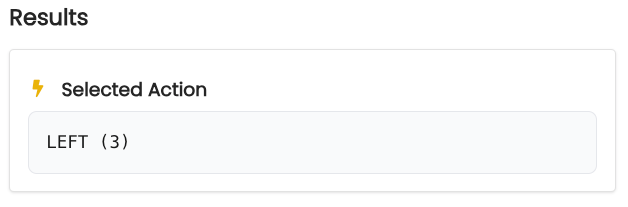
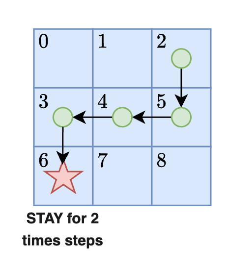
According to these results, the agent takes six total actions. It starts in position 2 (bulk storage) and moves to position 6 (packing station) where it stays until the end of the simulation. The figure below shows the agent's progression toward its goal. Once it reaches the goal square it stays there for two further time steps.
Each time we perform action selection the Genius agent will return information that reveals how the agent made its decision about which action to perform. This information is returned in both the model editor and Python SDK.
The action data reference page gives a more thorough analysis of all elements that are returned from action selection and their purpose.
For example, at any given time step we can calculate which state the agent thinks is most likely. We could also see the agent's evaluation of different policies at a given time step. Below we analyze the agent's behavior when in position 4 (convey)
When the agent is in position 4 (convey) it's belief state is:
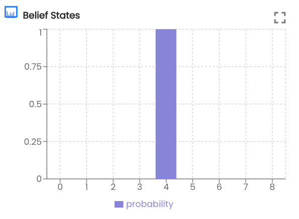
This indicates that the after receiving the belt observation the agent believes it is in the conveyer belt room. We can see that it has selected to move DOWN. Examining the action values we can see that DOWN was selected at the highest probability:
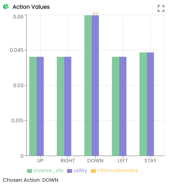
Inverse EFE and utility are explained in more detail in the multi-armed bandit tutorial. They do not apply in this simple agent navigation example.
First we import some convenience functions included in the SDK.
Next, we obtain the action result for time step 2 and extract the agent's belief and plot it.
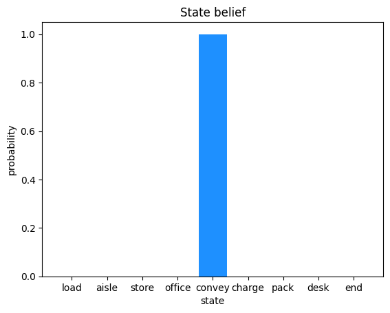
As we can see from the plot, the agent believes itself to be in the convey position in the warehouse. Next, we extract the policy belief from time step 2. The get_policy_space function enumerates all combinations of possible policies for a policy length of 2 given the 5 actions we have defined. The results are plotted.
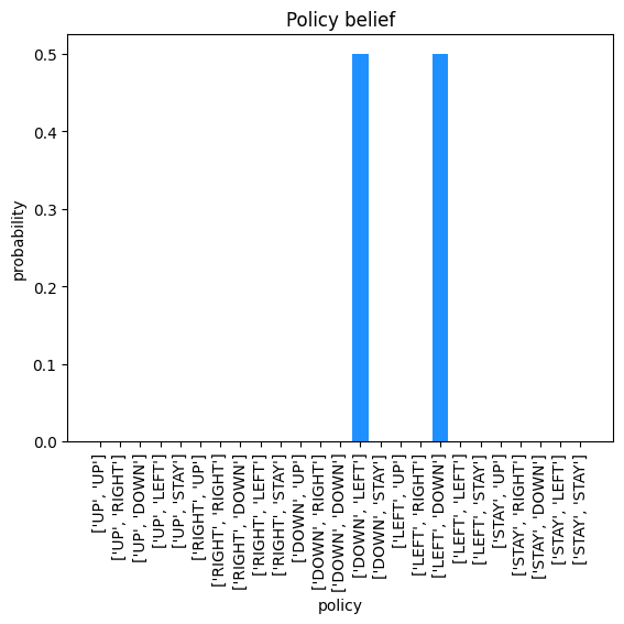
Here we can see that when the agent is in square 4 of the grid (convey) it believes that either sequence, DOWN then LEFT or LEFT then DOWN, will lead to its goal. In this case since the probabilities are tied, it will pick the first one (DOWN then LEFT) which is what we see in the results.
Last updated