
Python SDK
The Genius Python SDK enables users to build probabilistic models and query them directly in Python. This guide shows an overview of the different types of features provided by the SDK. For complete documentation visit the Python SDK reference section.
Installing the Python SDK
pip install genius-client-sdkImporting
The following lines can be used to import the main classes used in the SDK:
Genius model:
from genius_client_sdk.model import GeniusModelGenis agent:
from genius_client_sdk.agent import GeniusAgentPOMDP model:
from genius_client_sdk.pomdp import POMDPModel
Additional helper functions can be imported through the utils module:
from genius_client_sdk.utils import (
    control_map,
    flatten_nested_list,
    get_policy_space,
    onehot,
    plot_categorical,
    policy_map,
)Extra import
Other imported modules used by this quickstart
Connecting a Genius agent
Authentication
Before you begin, you need to choose an authentication method in order to connect to your Genius agent. These are the available options:
1. API Key
After importing Genius SDK in your python environment, you need to set up this credential:
2.Bearer Token (not available yet)
3.OAuth2 Client Credential (not available yet)
Agent
Once you have installed the Python SDK, you must connect it to a Genius agent. To connect to the Genius agent you must use agent's URL that was provided to you. For the purpose of example we will assume that the agent's URL is https://my.agent.hostname. When you initialize the agent, pass in the HTTP protocol, hostname, and port as follows:
Usually, the agent will raise an AssertionError or HTTP 401 if the credential is not valid.
Additionally, it is recommended to configure the logging so only necessary information is output:
Building a factor graph in Python
Genius models must be uploaded in JSON model format. One can type out the model in JSON format directly or, more conveniently, construct this JSON model in Python. We now demonstrate how to build a factor graph in Python using the GeniusModel class with the SDK, focusing on the simple sprinkler model introduced in the knowledge center:
sprinkler exampleAfter importing the GeniusModel class it must be initialized.
VFG(version='0.5.0', metadata=None, variables={}, factors=[], visualization_metadata=None)
At this point the model.vfg instance variable is empty because we have not added any variables or factors. The first step to building the model is to add the variables using the add_variable() class method. If you try to add factors first you will get an error. The variables must be specified with a name and the categories or values associated with that variable. We replicate the structure of the variables in the sprinkler model below.
VFG(version='0.5.0', metadata=None, variables={'cloudy': Variable(root=DiscreteVariableNamedElements(elements=['no', 'yes'], role=None)), 'rain': Variable(root=DiscreteVariableNamedElements(elements=['no', 'yes'], role=None)), 'sprinkler': Variable(root=DiscreteVariableNamedElements(elements=['off', 'on'], role=None)), 'wet_grass': Variable(root=DiscreteVariableNamedElements(elements=['no', 'yes'], role=None))}, factors=[], visualization_metadata=None)
If you wish to add a latent variable to your model, you can pass in an optional role="latent" argument to model.add_variable(). This will indicate to Genius that the variable is latent and therefore not available in any datasets used for training (parameter learning).
Now our variables have been added to the model so it is time to add factors. To add a factor you must specify:
A target variable for this factor
The parent(s) of this target variable (if any)
The probabilities associated with the target and parent variables.
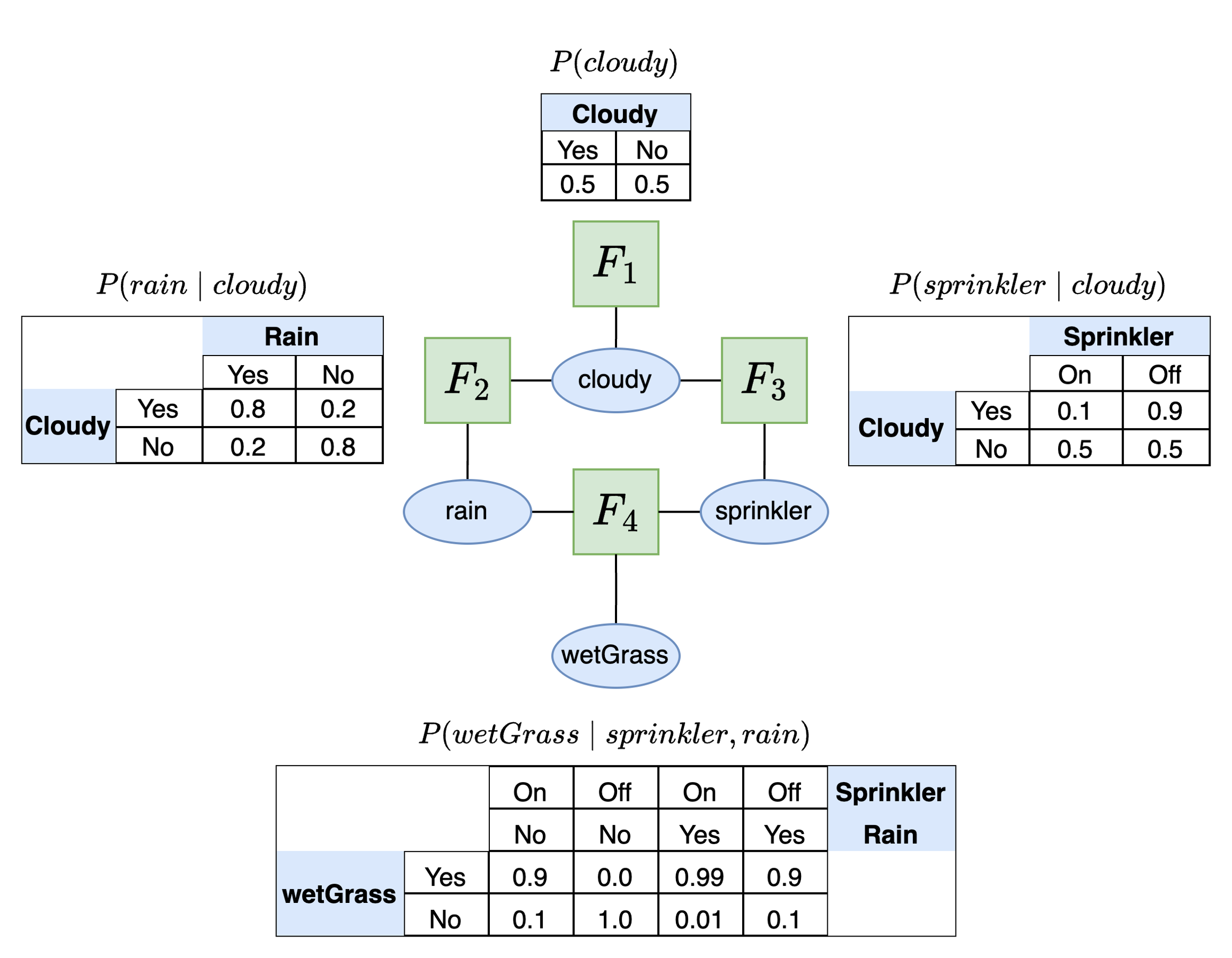
In the sprinkler example there are four possible factors. The table below lists the different target variables and parents for each factor:
P(cloudy)
cloudy
None
P(rain∣cloudy)
rain
cloudy
P(sprinkler∣cloudy)
sprinkler
cloudy
P(wetGrass∣rain,cloudy)
wetGrass
rain,cloudy
The first factor is a marginal distribution and thus has no parent as dependencies. The other distributions all have one or more parent variable that it depends on. The probability table associated with each factor is shown in the image above. First we specify the probabilities:
The dimensions of the probability table for a factor must correspond to the order of the variables that are associated with this factor. For example, if the factor is P(wetGrass∣rain,cloudy) then the dimensions of the factor probability table will have three dimensions. The first dimension will be the target variable (wetGrass), the second dimension will be the rain and the third dimension will be cloudy. This means that the target variable is always on the rows and the additional dimensions correspond to the parent variables in order.
Next, we add the probabilities, targets, and parents to the factor graph.
It is also possible to add "roles" to each factor which indicate a special function for this factor. This achieved through the role argument to the add_factor() method which accepts a string. These roles come into play when creating active inference models. The four possible role types are: "NoRole", "Transition", "Preference", "Likelihood" and "InitialStatePrior".
VFG(version='0.5.0', metadata=None, variables={'cloudy': Variable(root=DiscreteVariableNamedElements(elements=['no', 'yes'], role=None)), 'rain': Variable(root=DiscreteVariableNamedElements(elements=['no', 'yes'], role=None)), 'sprinkler': Variable(root=DiscreteVariableNamedElements(elements=['off', 'on'], role=None)), 'wet_grass': Variable(root=DiscreteVariableNamedElements(elements=['no', 'yes'], role=None))}, factors=[Factor(variables=['cloudy'], distribution=<Distribution.Categorical: 'categorical'>, counts=None, values=array([0.5, 0.5]), role=None), Factor(variables=['sprinkler', 'cloudy'], distribution=<Distribution.CategoricalConditional: 'categorical_conditional'>, counts=None, values=array([[0.5, 0.9],
[0.5, 0.1]]), role=None), Factor(variables=['rain', 'cloudy'], distribution=<Distribution.CategoricalConditional: 'categorical_conditional'>, counts=None, values=array([[0.8, 0.2],
[0.2, 0.8]]), role=None), Factor(variables=['wet_grass', 'sprinkler', 'rain'], distribution=<Distribution.CategoricalConditional: 'categorical_conditional'>, counts=None, values=array([[[1. , 0.1 ],
[0.1 , 0.01]],
[[0. , 0.9 ],
[0.9 , 0.99]]]), role=None)], visualization_metadata=None)
Before proceeding, it is important to validate your model to ensure that the structure and data types are correct. This can be achieved with the validate() class method:
Model validated successfully.
[]
Now save the model with the save() class method, specifying the outpath.
Finally, we can also visualize the model. This is a simple visual just to get an idea of what the factor graph looks like. For a better view it is recommended that the model is exported to JSON and loaded into the model editor.
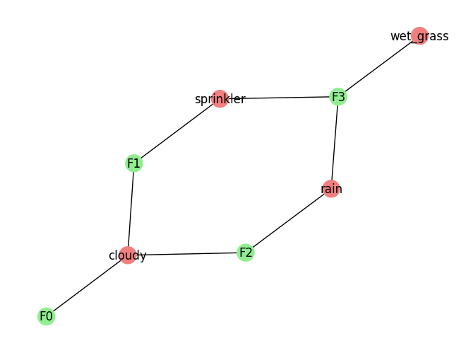
sprinkler factor graph structureExploring a Genius model's structure
The GeniusModel class comes equipped with a number of convenience functions that can be used to investigate the structure of the model. Running get_variable_names() will list all variables in the model:
['rain', 'sprinkler', 'wet_grass', 'cloudy']
Running get_variable_values(variable_id) and passing in a variable string from the list above will return the categories associated with that variable:
['no', 'yes']
['off', 'on']
Running get_factor_attributes(factor_id, attribute) and passing in an integer for the factor id of interest and the attribute to return will the desired properties of the factor. There are four possible attributes: the variables associated with the factor, the distribution type for the factor, the probability values associated with the factor, and the factor's role. In many cases a factor may have no role but in some cases, such as POMDP models, the factor may have a specific role of interest such as "likelihood" or (state) "transition".
['cloudy']
<Distribution.CategoricalConditional: 'categorical_conditional'>
array([[[1. , 0.1 ], [0.1 , 0.01]], [[0. , 0.9 ], [0.9 , 0.99]]])
None
Creating a Genius agent
To create a Genius agent, first initialize the class and connect to the agent.
Loading and viewing a model
There are two options available for loading a model.
Load a model from a JSON file path
To upload a model from a JSON file path, first ensure that your model is in the correct format. If JSON model is not available create one first in either the model editor or the Python SDK and then exported to JSON. Then run the following:
Load a model from an instance of GeniusModel
If you have already created a model using the GeniusModel class, as shown in the Building a Factor Graph in Python section above, then this model can be loaded into the Genius agent as follows:
To view the loaded model run:
{"version": "0.5.0","metadata": null,"variables": {"cloudy": {"elements": ["no","yes"],"role": null},"rain": {"elements": ["no","yes"],"role": null},"sprinkler": {"elements": ["off","on"],"role": null},
...
}],"visualization_metadata": null }
You can also pass in the optional argument summary=True to view a summary of the model contents in a more readable format:
Model contents:
4 variables: ['cloudy', 'rain', 'sprinkler', 'wet_grass']
4 factors: [['cloudy'], ['rain', 'cloudy'], ['sprinkler', 'cloudy'], ['wet_grass', 'sprinkler', 'rain']]

Factor probabilities:
[0.5 0.5]
[[0.5 0.9] [0.5 0.1]]
[[0.8 0.2] [0.2 0.8]]
[[[1. 0.1 ] [0.1 0.01]]
[[0. 0.9 ] [0.9 0.99]]]
Probabilistic inference
To perform probabilistic inference, use the infer(variable_id, evidence) method of the GeniusAgent class. This function can be used for conditioning or Bayesian inference. To infer the probability that the grass is wet given the evidence that it is raining and the sprinkler is off:
{'no': 0.10000000372529039, 'yes': 0.8999999962747096}
To perform Bayesian inference to invert a dependency relationship the same method is used:
{'no': 0.20628684298847688, 'yes': 0.7937131570115231}
Parameter learning
Parameter learning uses the learn() method of the GeniusAgent class. To perform parameter learning we have two options for input:
Import a CSV file
Provide the data in code
Parameter learning with CSV data
To use an existing CSV file as data for parameter learning first ensure that it is properly formatted with variable names as headers and rows of observations for each category corresponding to the variable. See the section on CSV data format for more details. Then run:
Learning successful. Use log_model() to see updated probabilities.
Parameter learning from Python
In the second instance, learning requires a list of strings for each variable name and a nested list of observations corresponding to each variable. For example:
Learning successful. Use log_model() to see updated probabilities.
There is no direct output from learning but the updated probabilities may be viewed using agent.log_model() or inspecting the dict stored in the agent.model instance variable.
Active inference
Active inference uses a special type of model known as a partially observable Markov decision process (POMDP). To construct a POMDP, one needs to define specific types of variables and factors. This is described in more detail in the active inference tutorial and agent navigation examples.
Creating a POMDP model
To create a POMDP model in the Python SDK we need to specify the following four factors:
Likelihood
Transition
State prior (optional)
Preference
In the active inference literature, these factors are usually referred to by single letter names for convenience. The likelihood is referred to as A, the state-transitions as B, the preferences as C, and the state prior as D.
We also need to specify the following three variables:
State
Observation (data)
Action
We are free to name these variable as we wish so that they correspond to the problem at hand. First, we initialize the POMDPModel() class so we can construct the POMDP model.
It is also possible to create a POMDP model with the GeniusModel class. However, the POMDPModel class provides some convenient helper functions to help construct the model.
Below, we show an example of a POMDP construction for the agent navigation example. First, we define some generic states and observations categories as the numbers 0-8.
We also define the possible actions the agent can take and the number of possible actions:
We will name the states as position and keep the names of the observations and actions as observation and action respectively. Now we add these variables to the model
First, we construct the likelihood. The likelihood connects states (position in this example) to observations.
The state transition connects the state at the current time step (position) with the state at the next time step (position) and also depends on the action performed.
The agent's preferences are defined in terms of the probability that it expects to receive a particular observation:
Finally, the optional state prior factor can be added:
Once the components are added, it is important to validate your model. If you are using the POMDPAgent class, then the validation will also check that all model components needed for a POMDP model are present.
Model validated successfully.
Action selection
To perform action selection, the agent needs to have a model loaded.
Next, we pass in an observation and a policy length. A policy is a sequence of actions the agent could take. Active inference agents plan their actions as sequences instead of individual actions so the policy length serves as "lookahead" to define how far into the future the agent will be planning. The following executes action selection:
Explainability and interpretability
The action_result contains a number of different pieces of information that reveal how the agent came to its decision and its beliefs about the state of the world. These pieces include:
The agent's belief about the unobserved state that it infers on the basis of the observation it receives.
The agent's belief over all policies under consideration given the actions and policy length.
The expected free energy (EFE) for each policy which is used by the agent to rank policies.
A break down of each component of EFE for each policy which indicates the type of behavior the agent is currently prioritizes (reward-seeking or exploratory).
A break down of EFE contributions for the currently selected actions.
For more detailed information on these components see the action data reference section.
Last updated